
Thử dùng AI Deepseek giúp viết hàm trong Google Sheets/Excel
Từ khi làn sóng AI bùng nổ với chatGPT, chắc hẳn ai cũng đã từng thử dùng AI cho một tác vụ nào đó trong đời sống rồi phải không? Trong bài viết này, Học Excel Online sẽ thử dùng AI Deepseek giúp viết hàm trong Google Sheets nhé.
Xem nhanh
AI Deepseek giúp viết hàm
Nếu các bạn vẫn còn lạ lẫm với cái tên này thì Deepseek là một mô hình AI đến từ trung quốc, được ra mắt và gây chú ý vào cuối năm 2024 bởi khả năng suy luận trước khi trả lời được tích hợp vào mô hình R1. Nói một cách đơn giản, thay vì đưa ra câu trả lời ngay, AI sẽ “suy nghĩ” trước, sẽ đưa ra các trường hợp, tự phản biện lại chính câu trả lời của mình… cho đến khi đưa ra phương án hợp lý nhất cho người dùng. Ứng dụng điều này trong thực tiễn, chúng ta sẽ có một “người” nghĩ cùng, đưa ra các phương án trước khi có giải pháp. Hãy cùng xem thử bài toán dưới đây:
Bài toán: Tạo thanh tra cứu trong Google Sheets
Mình có một bảng như sau:
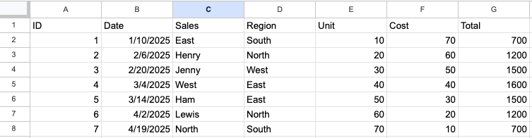
Bài toán ở đây đó là tạo một thanh tìm kiếm giúp nhanh chóng lọc dữ liệu theo các điều kiện và hiển thị. Ví dụ, nếu nhập vào thanh tìm kiếm cụm từ “Jenny”, lúc này chỉ dữ liệu của dòng thứ 3 được đưa ra.
Để giải quyết bài toán này với AI Deepseek, mình đưa ra những yêu cầu như sau:
Cụ thể prompt của mình:
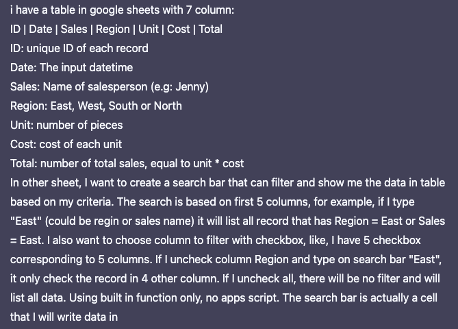
-Nhắc lại cấu trúc bảng: 7 cột, nội dung từng cột

-Yêu cầu tạo 1 thanh tìm kiếm để lọc dữ liệu, và thanh tìm kiếm sẽ sử dụng cho bất kỳ cột nào trong 5 cột đầu tiên. Ví dụ, nếu chọn cột Sales và điền “East” vào thanh tìm kiếm, chỉ dòng đầu tiên được hiển thị. Nhưng nếu ta chọn đồng thời cột Sales và Region sau đó điền “East” vào thanh tìm kiếm, ta sẽ nhận được kết quả là dòng 1, 4 và 5.
-Trong trường hợp không cột nào được chọn, tất cả dữ liệu sẽ được trả về.
-Thanh tìm kiếm được tạo bằng công thức, không sử dụng tới Google Apps Script.
_
Dưới đây là phản hồi của AI, thời gian suy nghĩ 253 giây:
Okay, let’s see. The user has a Google Sheets setup with a table of sales data and wants to create a search bar in another sheet that can filter the data based on input criteria. The search should check the first five columns (ID, Date, Sales, Region, Unit) but only those that are selected via checkboxes. If all checkboxes are unchecked, it shows all data. They want to use built-in functions only, no Apps Script.
First, I need to figure out how to create a dynamic filter based on the search term and the checkboxes. The checkboxes are likely linked to cells indicating TRUE (checked) or FALSE (unchecked). The search term is in a specific cell.
The main challenge is to check each row against the search term in the selected columns. For each row, if any of the selected columns contain the search term, that row should be included in the results.
Let’s break it down step by step.
1. **Checkbox Handling**: Each checkbox (probably in cells like B1:B5) corresponds to a column. When a checkbox is checked, that column should be included in the search. For example, if the Region checkbox is checked, the formula should check the Region column for the search term.
2. **Search Term**: The user types the search term into a specific cell, say A1. The formula needs to reference this cell.
3. **Filter Function**: Use the FILTER function to display the results. But the condition for FILTER needs to dynamically check each selected column for the search term.
4. **Dynamic Condition**: For each row, create a condition that checks if the search term exists in any of the selected columns. For each column, if the checkbox is checked, check if the search term matches that column’s data. Then combine these with OR logic.
5. **Handling Data Types**: Some columns are numbers (ID, Unit) and others are text (Date as datetime, Sales, Region). The search term is text, so when searching in numeric columns, we might need to convert them to text for comparison. For example, if the user searches “123”, it should match an ID of 123.
6. **Case Insensitivity**: The search should be case-insensitive. Using LOWER on both the search term and the column data can help with that.
7. **Date Handling**: If the Date column is a datetime, converting it to text might be tricky. Using TEXT(date_column, “yyyy-mm-dd hh:mm:ss”) can standardize the format for comparison.
Putting it all together:
– For each column (ID, Date, Sales, Region, Unit), check if the checkbox is TRUE.
– For each checked column, check if the search term (lowercase) is in the lowercase version of the column’s data (converted to text).
– Combine these checks with OR.
– Apply this combined condition to the FILTER function to get the matching rows.
So, the formula structure would be something like:
=FILTER(Data!A:G,
( (Checkbox_ID = TRUE) * (LOWER(TO_TEXT(Data!A:A)) = LOWER(search_term)) +
( (Checkbox_Date = TRUE) * (LOWER(TEXT(Data!B:B, “yyyy-mm-dd hh:mm:ss”)) = LOWER(search_term)) ) +
… and so on for other columns … > 0 )
But wait, adding the conditions with + acts as an OR because if any is TRUE (1), the sum is greater than 0. However, multiplication (*) is used for AND logic here between the checkbox and the column condition.
But actually, each term is (Checkbox * Condition), which would be 1 if both are TRUE. Summing all those terms gives the number of columns where both the checkbox is checked and the condition is met. If the sum is >=1, then the row is included.
But the user wants to check if the search term is in ANY of the checked columns. So for each row, we check each column if it’s checked and matches the term, then OR those results.
Alternatively, using REGEXMATCH might be another approach, but handling each column separately with checkboxes seems more straightforward.
Another consideration: the Data sheet might have headers, so we should exclude the header row in the filter. So, using A2:G instead of A:G, and adjusting the ranges accordingly.
Also, handling empty search term: if the search term is empty, but checkboxes are checked, should it show all rows? But according to the user’s requirement, if all checkboxes are unchecked, it shows everything. If some are checked and the search term is empty, then it’s equivalent to searching for empty string in those columns. But the user probably wants that if the search term is empty, no filtering is applied, regardless of checkboxes. Hmm, but the user says if all checkboxes are unchecked, show all. If checkboxes are checked and search term is empty, maybe it shows all rows where any of the checked columns are empty? That might not be intended. The user’s requirement is that the search is based on the term and the checkboxes. So if the search term is empty, even with checkboxes checked, perhaps it shows all data. But the original problem states that if all checkboxes are unchecked, it lists all data. So maybe the checkboxes only determine which columns to check, but if the search term is empty, it doesn’t filter. Let me recheck the user’s question.
The user says: “if I uncheck all, there will be no filter and will list all data.” So if all checkboxes are unchecked, regardless of the search term, it shows all. But if any checkboxes are checked, then it filters based on the search term in those columns. Also, if the search term is empty, even with checkboxes checked, it would look for empty strings in those columns. But the user probably wants that when the search term is empty, and checkboxes are checked, it doesn’t filter. However, that’s not explicitly stated.
Assuming that the search only applies when there’s a search term. If the search term cell is empty, then no filtering is done. But the user’s current setup doesn’t mention that. So perhaps the formula needs to account for both the checkboxes and the presence of a search term.
Alternatively, the formula will always check the search term against the checked columns. So if the search term is empty, it would look for rows where any of the checked columns are empty. That might not be desired. To avoid that, we can add a condition that if the search term is empty, it returns all rows (if any checkboxes are checked, but maybe not). Wait, this is getting complicated.
But according to the user’s problem statement: the search bar is a cell where they type the criteria. So when they type “East”, it checks the columns. If they clear the search bar, it should show all data again. Therefore, if the search term is empty, regardless of checkboxes, it shows all data. That makes sense. So the formula should check that the search term is not empty before applying the filters. If the search term is empty, return all data. If checkboxes are all unchecked, return all data. Otherwise, apply the filters.
So combining these conditions:
If the search term is empty OR all checkboxes are unchecked, show all data. Otherwise, filter based on the search term in checked columns.
So the formula would have a condition that checks:
IF( OR(search_term = “”, AND(all checkboxes are FALSE)),
Data!A2:G,
FILTER(Data!A2:G, [conditions based on checkboxes and search term]) )
But how to implement this with built-in functions?
Alternatively, structure the FILTER’s condition to account for these cases.
But perhaps using a helper formula to determine whether to apply the filter or not.
But let’s proceed step by step.
Let’s assume:
– Search term is in cell A1 of the second sheet.
– Checkboxes for the five columns (ID, Date, Sales, Region, Unit) are in cells B1:B5, with B1=ID, B2=Date, etc., each linked to a checkbox, so B1 is TRUE when checked.
– The data is in Data!A2:G (assuming row 1 is headers).
The formula needs to:
1. If A1 is empty, return all data.
2. If all checkboxes (B1:B5) are FALSE, return all data.
3. Else, for each row in Data, check if any of the checked columns contain the search term (exact match? or partial? The user example shows “East” matching Region=East or Sales=East, which is exact. But maybe it’s better to allow partial matches. Wait, the user example says if you type “East” it lists records where Region = East or Sales = East. So exact match. But maybe the user wants partial matches. The question isn’t clear. Let’s assume exact match for now, but if the user wants partial, we can adjust with SEARCH or FIND functions.)
But the user’s example uses “East” to match Region = East. So exact match. So we need to check if the cell’s content equals the search term.
But considering case insensitivity, “east” should also match “East”. So convert both to lowercase.
So, for each column:
If the checkbox is TRUE, check if LOWER(Data!column) = LOWER(search_term).
But for columns like Date (which is a datetime), converting to text might be necessary. For example, if the user types “2023-10-05”, it should match the date in the Date column. So converting the date to a text string in a specific format would help. Using TEXT(Data!B2, “yyyy-mm-dd hh:mm:ss”) to standardize the date format.
Similarly, numeric columns like ID and Unit should be converted to text for comparison. For example, ID 123 as text “123”.
So, the formula for each column’s condition would be:
For ID (column A):
IF(B1=TRUE, LOWER(TO_TEXT(Data!A2:A)) = LOWER($A$1), FALSE)
Similarly for Date (column B):
IF(B2=TRUE, LOWER(TEXT(Data!B2:B, “yyyy-mm-dd hh:mm:ss”)) = LOWER($A$1), FALSE)
For Sales (column C):
IF(B3=TRUE, LOWER(Data!C2:C) = LOWER($A$1), FALSE)
For Region (column D):
IF(B4=TRUE, LOWER(Data!D2:D) = LOWER($A$1), FALSE)
For Unit (column E):
IF(B5=TRUE, LOWER(TO_TEXT(Data!E2:E)) = LOWER($A$1), FALSE)
Then, combine these five conditions with OR logic. In Google Sheets, addition of the conditions (since each is 0 or 1) would act as OR. So:
(condition_ID + condition_Date + condition_Sales + condition_Region + condition_Unit) > 0
So the overall FILTER condition would be:
=IF(OR($A$1=””, COUNTA(B1:B5)=0), Data!A2:G,
FILTER(Data!A2:G,
(IF(B1=TRUE, LOWER(TO_TEXT(Data!A2:A)) = LOWER($A$1), 0) +
(IF(B2=TRUE, LOWER(TEXT(Data!B2:B, “yyyy-mm-dd hh:mm:ss”)) = LOWER($A$1), 0) +
(IF(B3=TRUE, LOWER(Data!C2:C) = LOWER($A$1), 0) +
(IF(B4=TRUE, LOWER(Data!D2:D) = LOWER($A$1), 0) +
(IF(B5=TRUE, LOWER(TO_TEXT(Data!E2:E)) = LOWER($A$1), 0)) > 0))
But in Google Sheets, you can’t use IF inside FILTER’s condition like that. Instead, you need to use array formulas for each condition.
Wait, perhaps using multiplication:
For each column, the condition is (Checkbox) * (ColumnData = SearchTerm). Then sum all these, and if the sum is >=1, include the row.
But since the checkboxes are in individual cells (B1 to B5), which are single cells (not arrays), we can reference them as B$1, B$2, etc.
Wait, but in an array formula, B$1 is a scalar, so when multiplied by an array, it applies to all elements.
So, let’s construct each column’s condition as:
(B$1) * (LOWER(TO_TEXT(Data!A2:A)) = LOWER($A$1)) +
(B$2) * (LOWER(TEXT(Data!B2:B, “yyyy-mm-dd hh:mm:ss”)) = LOWER($A$1)) +
… and so on.
But in Google Sheets, you can’t mix array and non-array operations like that without ARRAYFORMULA.
Therefore, wrapping everything in ARRAYFORMULA.
But the FILTER function can handle array conditions.
Alternatively, construct the condition using ARRAYFORMULA.
Wait, let’s try writing the formula step by step.
Assume:
– Search term is in cell A1 of the second sheet.
– Checkboxes are in B1 (ID), B2 (Date), B3 (Sales), B4 (Region), B5 (Unit).
The formula in the second sheet where results should appear (starting from A2, for example):
=IF(OR(A1=””, AND(B1:B5=FALSE)), Data!A2:G,
FILTER(Data!A2:G,
ARRAYFORMULA(
(B1 * (LOWER(TO_TEXT(Data!A2:A)) = LOWER(A1))) +
(B2 * (LOWER(TEXT(Data!B2:B, “yyyy-mm-dd hh:mm:ss”)) = LOWER(A1)) +
(B3 * (LOWER(Data!C2:C) = LOWER(A1))) +
(B4 * (LOWER(Data!D2:D) = LOWER(A1))) +
(B5 * (LOWER(TO_TEXT(Data!E2:E)) = LOWER(A1)))
> 0))
))
But let’s check this:
Each term like (B1 * …) uses B1 as TRUE (1) or FALSE (0). If B1 is TRUE, then the corresponding column’s condition is checked. Each condition is an array (per row) comparing the column’s data to the search term. Multiplying by B1 effectively enables or disables that condition.
Adding all these terms gives, for each row, the number of checked columns where the search term matches. If the sum is >0, the row is included.
This should work. However, there are some potential issues:
1. **Date Handling**: If the Date column (B) is a valid date, TEXT(Data!B2:B, “yyyy-mm-dd hh:mm:ss”) converts it to a string. If the user enters a date in a different format, like “10/05/2023”, it won’t match. So the user must input the date in the exact format used in the TEXT function. Alternatively, use different formats, but that complicates things. The user needs to be aware of the expected format.
2. **Numeric to Text Conversion**: For ID and Unit columns, converting numbers to text ensures that searching for “123” matches the numeric 123. However, if the user inputs a number with decimals or formatting (like “123.00”), it might not match. Using TO_TEXT should handle integers correctly.
3. **Case Insensitivity**: Converting both the search term and column data to lowercase ensures case insensitivity.
4. **Empty Search Term**: The formula checks if A1 is empty or all checkboxes are unchecked, in which case it returns all data.
But wait, in the initial IF condition, it’s OR(A1=””, AND(B1:B5=FALSE)). If either the search term is empty OR all checkboxes are unchecked, show all data. But the user’s requirement is that if all checkboxes are unchecked, regardless of the search term, show all data. Also, if the search term is empty, regardless of checkboxes, show all data. That seems to align with the formula.
But wait, the user says: “If I uncheck all, there will be no filter and will list all data.” So even if there’s a search term, if all checkboxes are unchecked, it lists all data. So the formula correctly includes that in the OR condition.
Another edge case: if some checkboxes are checked, but the search term is empty, then the formula would return all data, because A1 is empty. Which is correct.
Now, putting this into the formula:
=IF(OR(A1=””, AND(B1:B5=FALSE)), Data!A2:G,
FILTER(Data!A2:G,
ARRAYFORMULA(
(B1 * (LOWER(TO_TEXT(Data!A2:A)) = LOWER(A1)) +
B2 * (LOWER(TEXT(Data!B2:B, “yyyy-mm-dd hh:mm:ss”)) = LOWER(A1)) +
B3 * (LOWER(Data!C2:C) = LOWER(A1)) +
B4 * (LOWER(Data!D2:D) = LOWER(A1)) +
B5 * (LOWER(TO_TEXT(Data!E2:E)) = LOWER(A1))
) >0))
)
But in Google Sheets, the AND function doesn’t work on ranges like AND(B1:B5=FALSE). Instead, we can check if the count of TRUEs is zero. COUNTA(B1:B5) counts the number of checked checkboxes (assuming that when a checkbox is checked, the cell is TRUE). Wait, no: COUNTA counts non-empty cells. If the checkboxes are linked to B1:B5, then when checked, they are TRUE, which is counted by COUNTA. But to count how many are checked, we can use COUNTIF(B1:B5, TRUE). If COUNTIF(…)=0, then all are unchecked.
So the initial condition should be:
IF(OR(A1=””, COUNTIF(B1:B5, TRUE)=0), Data!A2:G, FILTER(…))
So adjusting the formula:
=IF(OR(A1=””, COUNTIF(B1:B5, TRUE)=0), Data!A2:G,
FILTER(Data!A2:G,
ARRAYFORMULA(
(B1*(LOWER(TO_TEXT(Data!A2:A))=LOWER(A1)) +
B2*(LOWER(TEXT(Data!B2:B, “yyyy-mm-dd hh:mm:ss”))=LOWER(A1)) +
B3*(LOWER(Data!C2:C)=LOWER(A1) +
B4*(LOWER(Data!D2:D)=LOWER(A1)) +
B5*(LOWER(TO_TEXT(Data!E2:E))=LOWER(A1))
)>0))
)
Wait, but in the formula, the multiplication is between B1 (a single cell) and an array (result of the condition). So when B1 is TRUE (1), it multiplies each element of the condition array by 1, otherwise by 0. Then summing all such terms for each row. If the sum is >0, include the row.
Yes, this should work.
Testing with sample data:
Suppose Data!A2:E has:
ID | Date | Sales | Region | Unit
1 | 2023-10-05 10:00 | Jenny | East | 5
If search term is “East”, and Region checkbox (B4) is checked, then the condition for Region is TRUE, so the row is included.
If Region is unchecked and Sales is checked, and the search term is “Jenny”, it’s included.
If the search term is “east” (lowercase), with Region checked, it still matches because of LOWER.
Date example: If the user enters “2023-10-05 10:00:00” and Date checkbox is checked, it matches. But if the date is displayed differently, the user must input the exact format.
Potential issues:
– The date format must match exactly what’s produced by the TEXT function. If the user inputs “05-10-2023”, it won’t match. So the user needs to input dates in “yyyy-mm-dd hh:mm:ss” format.
– Numeric fields must be input as exact numbers. For example, if the user searches “5” and Unit is 5, it matches. If Unit is 5.0, TO_TEXT might convert to “5” as well, so it should still match.
Another thing: TO_TEXT(Data!A2:A) converts numbers to text, so “00123” would match 123 if the ID is numeric, but if the ID is stored as text with leading zeros, it would matter. So if IDs are numeric, searching for “123” would match the numeric ID 123, but if stored as text “0123”, it wouldn’t. So the user should ensure data types are consistent.
Now, putting all this together in the formula.
Also, the user might have headers in the Data sheet, so the formula should start from row 2. The FILTER function in the formula uses Data!A2:G, assuming data starts at row 2.
Finally, the formula would be:
=IF(OR(A1=””, COUNTIF(B1:B5, TRUE)=0), Data!A2:G,
FILTER(Data!A2:G,
ARRAYFORMULA(
(B1*(LOWER(TO_TEXT(Data!A2:A))=LOWER(A1)) +
B2*(LOWER(TEXT(Data!B2:B, “yyyy-mm-dd hh:mm:ss”))=LOWER(A1)) +
B3*(LOWER(Data!C2:C)=LOWER(A1)) +
B4*(LOWER(Data!D2:D)=LOWER(A1)) +
B5*(LOWER(TO_TEXT(Data!E2:E))=LOWER(A1))
)>0))
)
Make sure to adjust the ranges (A2:A, B2:B, etc.) to match the actual data range. If the data has 1000 rows, better to use Data!A2:A1000, etc., to avoid processing entire columns which can slow down the sheet.
Alternatively, use Data!A2:G where G is the last column, but again, it’s better to limit the range to the actual data size.
So, the final formula the user should enter in their search results sheet is:
=IF(OR(A1=””, COUNTIF(B1:B5, TRUE)=0), Data!A2:G,
FILTER(Data!A2:G,
ARRAYFORMULA(
(B1*(LOWER(TO_TEXT(Data!A2:A))=LOWER(A1)) +
B2*(LOWER(TEXT(Data!B2:B, “yyyy-mm-dd hh:mm:ss”))=LOWER(A1)) +
B3*(LOWER(Data!C2:C)=LOWER(A1)) +
B4*(LOWER(Data!D2:D)=LOWER(A1)) +
B5*(LOWER(TO_TEXT(Data!E2:E))=LOWER(A1))
)>0))
)
Note: Ensure that the checkboxes are linked to cells B1 to B5, and the search term is in cell A1. Adjust cell references as needed based on the actual setup.
Another consideration: If the data in the Date column is stored as text, the TEXT function might not be necessary, but if it’s a valid date, the TEXT function is essential to convert it to a comparable string.
Finally, the user may need to adjust the date format in the TEXT function to match how they input dates. For example, if they input dates as “mm/dd/yyyy”, the TEXT function should use “mm/dd/yyyy hh:mm:ss” instead.
Sau đó, Deepseek đã hướng dẫn setup và đưa cho mình công thức:
=IF(OR(A1="", COUNTIF(B1:B5, TRUE)=0), Data!A2:G,
FILTER(Data!A2:G,
 ARRAYFORMULA(
  (B1*(LOWER(TO_TEXT(Data!A2:A))=LOWER(A1)) +
  B2*(LOWER(TEXT(Data!B2:B, "yyyy-mm-dd hh:mm:ss"))=LOWER(A1)) +
  B3*(LOWER(Data!C2:C)=LOWER(A1)) +
  B4*(LOWER(Data!D2:D)=LOWER(A1)) +
  B5*(LOWER(TO_TEXT(Data!E2:E))=LOWER(A1))
 )>0))
Với A1 là nơi chúng ta sẽ đặt làm thanh tìm kiếm, từ ô B1 tới B5 sẽ thiết lập các checkbox tương ứng với 5 cột ID, Date, Sales, Region và Unit. Công thức sẽ được đặt ở 1 ô ngoài những ô trên, ví dụ như B8. Dữ liệu của chúng ta nằm trong Sheet “Data”.
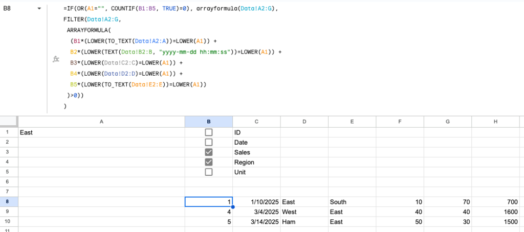
Khi thử kiểm tra, công thức trên chỉ sai duy nhất một chỗ: Data!A2:G. Bởi Google Sheets không tự động mở rộng công thức như Excel, mà ta cần thêm vào INDEX hoặc ARRAYFORMULA. Sau khi thêm phần còn thiếu, công thức đã hoạt động hoàn toàn bình thường và chính xác.
Các bạn có thể xem và tải về file tại đây: https://docs.google.com/spreadsheets/d/1MqfL_dT6saBXEj2HRkIkA9HPT61imTMsX6gUF3HTulg/edit?usp=sharing


